Coder Corner

Part 6b – less cache misses

Last time we took care of our input data, and packed it in a nice flat linear array. This is necessary but not sufficient to guarantee high performance: it only helps if you actually read that input array sequentially. But if you read random boxes within the input array, you still get cache misses.

But do we still get cache misses? We got great speedups with our previous change so aren’t we done? How do we know if there is more to gain from “the same” optimization?

One way is simply to look at the code. With some experience you can relatively easily spot the potential problems and “see” if the code is sound or not.

Another way would be to use a profiler like V-Tune, and check how many cache misses you get in that function.

And sometimes you can simply design small experiments, small tests that artificially remove the potential problems. If the performance doesn’t change, then you know you’re good, nothing left to do. If the performance does change, then you know you have some more work ahead of you.

This probably sounds a bit abstract so let me show you what I mean. The code is like this now:

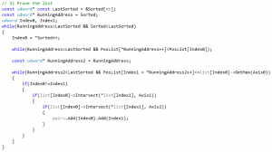
So we’re going to read from this badly-named “list” array. We look for “list” in the code. We first find this:

This reads the array sequentially, this is theoretically optimal, so no problem here. Granted: we don’t use all the data in the cache line we just fetched, but let’s ignore this. For now we are just checking whether we read the array sequentially or in random order.

Next we find this:

With:

And “Sorted” is the output of the radix sort, which sorted boxes along the X axis.

Well this one is not good. The radix implementation is for a “rank sorter”, i.e. it returns sorted indices of input bounds. But it does not sort the input array itself (contrary to what std::sort would do, for example). This means that we keep reading random boxes in the middle of the box-pruning loop. Oops.

And the same problem occurs for Index1 later on:

So this is what I mentioned above: you read the code, and you can easily spot theoretical problems.

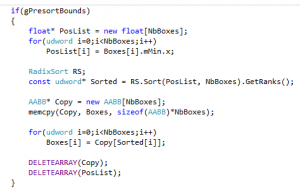
And then you can sometimes design tests to artificially remove the problem and see if performance changes. In this case we’re lucky because it’s easy to do: we can just pre-sort the input array (the bounds) before calling the box-pruning function. That way the sorting inside the function will have no effect, the radix sort will return an identity permutation, the code will read the input array sequentially, and we will see how much time we waste in cache misses.

Quickly said, quickly done, the change is just like this in Main.cpp:

Change gPresortBounds from false to true, run the test again… and….

Home PC:

Complete test (brute force): found 11811 intersections in 355897 K-cycles.

Complete test (box pruning): found 11811 intersections in 46586 K-cycles.

Office PC:

Complete test (brute force): found 11811 intersections in 312868 K-cycles.

Complete test (box pruning): found 11811 intersections in 49315 K-cycles.

Wo-ah.

Now that’s interesting. The function became faster again. This means that we are still suffering from cache misses out there, and that there is more to do to address this issue.

It is also a great example of why data-oriented design matters: the code did not change at all. It is the exact same function as before, same number of instructions, same position in the executable. It computes the same thing, returns the same number of overlapping pairs.

But somehow it’s 15% / 20% faster, just because we reorganized the input data. Ignore this, focus only on the code, and that’s the amount of performance you leave on the table in this case.

On a side note, we saw this kind of things in the past, in different contexts. For example triangle lists reorganized to take advantage of the vertex cache were faster to render - sometimes faster than strips. Even on older machines: making the code run faster by just changing the data is very reminiscent of what Leonard / Oxygene reported when working on his 16*16 “sprite record” demos on Atari ST. Several times in these experiments the Atari ST code didn’t change at all, but he was able to display more and more sprites by improving his “data builder” (a tool running on a PC). This had nothing to do with cache misses, but it was the same observation: you get the best results by optimizing both the code and the data. In his case, the data was not even optimized on the same machine/architecture.

So, anyway: we identified the problem. Now how do we solve it?

Well, the obvious way: we just create a secondary bounds array, sorted in the desired order, and we parse that sorted array instead of the original one. Basically we simply replicate what we did above to presort bounds, inside the box pruning function.

So, yes, we need more memory. And yes, the setup code becomes more complex (but it was not the bottleneck at all, remember? So it doesn’t matter).

On the other hand, now that the array itself is sorted, there is no need to work with the sorted indices anymore: they will always be the identity permutation. So the setup code becomes more complex but the inner loop’s code can actually be further simplified.

One complication is that we need to introduce a remapping between the user’s box indices and our now entirely sequential internal box indices. Fortunately we already have the remap table: it is the same as the sorted indices returned by the radix sort! So it all fits perfectly together and the only thing we need to do is remap the box indices after an overlap has been found, before writing them to the output buffer. In other words: we removed indirections in the frequent case (for each parsed box), and added indirections in the infrequent case (when an overlap is actually found).

The results speak for themselves.

Home PC:

Complete test (brute force): found 11811 intersections in 781350 K-cycles.
45584 K-cycles.
44734 K-cycles.
41679 K-cycles.
41810 K-cycles.
41654 K-cycles.
41623 K-cycles.
41634 K-cycles.
41605 K-cycles.
41779 K-cycles.
41633 K-cycles.
42037 K-cycles.
41752 K-cycles.
41836 K-cycles.
41639 K-cycles.
41618 K-cycles.
41636 K-cycles.
Complete test (box pruning): found 11811 intersections in 41605 K-cycles.

Office PC:

Complete test (brute force): found 11811 intersections in 813615 K-cycles.
46985 K-cycles.
46282 K-cycles.
47889 K-cycles.
47757 K-cycles.
55044 K-cycles.
52660 K-cycles.
47923 K-cycles.
53199 K-cycles.
47410 K-cycles.
46192 K-cycles.
45860 K-cycles.
46140 K-cycles.
45634 K-cycles.
46274 K-cycles.
47077 K-cycles.
46284 K-cycles.
Complete test (box pruning): found 11811 intersections in 45634 K-cycles.

The gains are summarized here:

This is even faster than what we got during our previous experiment with pre-sorted bounds. Which means that not only we took care of the cache misses, but also the extra simplifications of the main loop provided additional gains. Bonus!

And with that, we became 2X faster than the version we started from. That’s a milestone.

What we learnt:

The same as in the previous post, but it’s so important it’s worth repeating: cache misses are more costly than anything else. If you can only optimize one thing, that’s what you should focus on.

Before we wrap this one up, let’s come back to the loss of genericity we mentioned before. At the end of part 5 we said that we could get back our generic version for no additional cost. That is, we could put back the user-defined axes and don’t pay a performance price for it.

It should be clear why this is the case. We are now parsing internal buffers in the main loop, instead of the user-provided source array. So we could very easily flip the box coordinates while filling up these internal buffers, in the setup code. The main inner loop would remain untouched, so it would give back the user-defined axes virtually for free.

So that’s one loose end taken care of. But there is another big one left, also mentioned in part 5: SIMD.

We will slowly move towards it in next post.

GitHub code for part 6b

Part 6a – data-oriented design

There has been a lot of talks and discussions in the past about “data-oriented programming” and how it leads to faster code. Just Google the term along with “Mike Acton” and you will find plenty of it. I don’t need to repeat everything here: Mike is right. Listen to Mike.

In practical terms: we need to think about cache misses now. What we do with the data is one thing, but how we access the data is another equally important thing.

As far as our box pruning function is concerned, the data is pretty simple: we read an array of AABB pointers in input, and we write an array of pairs in output.

Reading from and writing to linear arrays is the most cache-friendly thing one can do, so we’re not starting from a bad place (there is no linked lists or complicated structures here). However we are reading an array of AABB pointers, not an array of AABBs. And that extra indirection is probably costly.

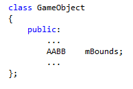
I remember using this design for practical reasons: I wanted the function to be user-friendly. At the time I was using a classical “object-oriented” design for my game objects, and I had something like this:

The AABB of each object was embedded within the game object class, vanilla C++ design. And I didn’t want the library to force users to first gather and copy the bounds in a separate bounds array just to be able to call the function. So instead, the function accepts an array of AABB pointers, so that it can read the AABBs directly from the game objects. The AABBs can neatly stay as a member of the objects, there is no need to duplicate them in a separate array and use more memory, no need to break up the neat objects into disjoint classes, it all looked quite nice.

And I suppose it was. Nice.

But fast, no, that, it was not.

Reading the bounds directly from the game objects is an extraordinarily bad idea: it makes you read some scattered data from some random location for each box, it’s the perfect recipe for cache misses and basically the worst you can do.

You can solve it with prefetch calls, to some extents. But prefetching is a fragile solution that tends to break when code gets refactored, and making it work in a cross-platform way is tedious (the different platforms may not even have the same cache line size, so you can easily imagine the complications).

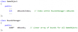
A better idea is to switch to “data-oriented design” instead of “object-oriented design”. In our case it simply means that the bounds are extracted from the game objects and gathered in an array of bounds, typically called “bounds manager”. Something along these lines:

Vanilla data-oriented design, that one.

There are pros & cons to both approaches, which are beyond the scope of this blog post. All I am concerned about here is the performance of the box pruning function, and in this respect the data-oriented design wins big time.

The modifications to the code are minimal. The function signature simply becomes:

And the corresponding indirections are removed from the code. That’s it. That’s the only difference. We don’t “optimize” the code otherwise. But the effect on performance is still dramatic:

Home PC:

Complete test (brute force): found 11811 intersections in 782034 K-cycles.
64260 K-cycles.
60884 K-cycles.
60645 K-cycles.
60586 K-cycles.
60814 K-cycles.
62650 K-cycles.
60591 K-cycles.
60697 K-cycles.
60833 K-cycles.
60579 K-cycles.
60601 K-cycles.
60905 K-cycles.
60596 K-cycles.
60836 K-cycles.
60673 K-cycles.
60585 K-cycles.
Complete test (box pruning): found 11811 intersections in 60579 K-cycles.

Office PC:

Complete test (brute force): found 11811 intersections in 810333 K-cycles.
59420 K-cycles.
58451 K-cycles.
59005 K-cycles.
65448 K-cycles.
64930 K-cycles.
62007 K-cycles.
59005 K-cycles.
58847 K-cycles.
58904 K-cycles.
58462 K-cycles.
58843 K-cycles.
58655 K-cycles.
58583 K-cycles.
59056 K-cycles.
58776 K-cycles.
58556 K-cycles.
Complete test (box pruning): found 11811 intersections in 58451 K-cycles.

The gains are summarized here:

The modifications to the code have been the smallest so far (really just replacing “->” with “.” here and there), and yet this gave the biggest speedup until now. In other words: our current best optimization did not come from modifying how we process the data (==roughly, “the code”), or from changing the data itself, but instead it came from changing how we access the data. That’s a pretty powerful result.

What we learnt:

Choose data-oriented design over object-oriented design for performance.

The data access pattern is often more important than anything else.

We are not done yet though. There is a lot more to do w.r.t. optimizing our data access, as we will see next time. But this change was so small and yet so effective that it was worth isolating in a separate blog post to drive the point home.

GitHub code for part 6a

Part 5 – hardcoding

Last time we saw how making the code less generic could also make it faster. This trend continues in this post.

There is another part of the box-pruning function that looks suspiciously over-generic. In the original code the sorting axes are defined by the user and sent as a parameter to the function:

In the initial code from 2002, I passed the following axes to the function:

Inside the function they are copied to local variables:

After that, the boxes are sorted along the main axis (Axis0), which essentially replicates the X-related part of the AABB::Intersect(const AABB& a) function. In other words, the sorting and scanning procedure emulates this line from AABB::Intersect():

And the remaining AABB::Intersect() tests for Y and Z are implemented using the remaining Axis1 and Axis2 variables:

This is all good and fine. Unfortunately it is also sub-optimal.

It was invisible to me when I first wrote the code, but I know now that fetching the axes from user-defined variables has a measurable impact on performance. I saw it happen multiple times in multiple algorithms. The cost is not always large, but it is always real: fetching the axes is going to be either an extra read from the stack, or one less register available to the optimizer to do its job - and there aren’t a lot of registers in the first place on x86. Either way it makes the addressing mode more complex, and if all these things happen in the middle of an inner loop, it quickly accumulates and becomes measurable.

So a much better idea is simply to hardcode the axes.

Well, a more efficient idea at least. Whether it is “better” or not is debatable.

Let’s see the effect on performance first, and debate later.

So the function sorted the boxes along X, and then did extra overlap tests on Y and Z within the most inner loop. The rationale for this default choice was that the up axis is usually either Y or Z, “never” X. You typically don’t want to sort along your up axis, because most games have a flat, essentially 2D world, even if they’re 3D games. If you project the bounds of such a world along the up axis, the projections will pretty much all overlap each-other, and this will greatly reduce the “pruning power” of the main sort. Basically the algorithm would then degenerate to the O(n^2) brute-force version.

Thus, the safest main sorting axis is X, because it is usually not the vertical axis. After that, and for similar reasons, it is usually slightly better to use the remaining non-vertical axis for “Axis1″ and keep the vertical axis last in “Axis2″ (the 2D overlap test can then early-exit more quickly).

One can also analyze the distribution of objects at runtime and select a different main axis each frame, depending on how objects are spatially organized at any given time. That’s what I did in my old Z-Collide library, eons ago.

Similarly, one could try to make the code more generic by removing the requirements that the input axes are the regular X, Y, Z coordinate axes. After all it is perfectly possible to project the boxes along an arbitrary 3D axis, so the main sorting axis could be anything, and the remaining other two axes could be derived from it in the same way a frame can be derived from just a view vector. Unfortunately making the code more generic in such a way, while “better” in theory (because the main sorting axis could be “optimal”), is a terrible idea in practice. You need to introduce dot-products to project the boxes instead of directly reading the bounds’ coordinates, it adds a lot of overhead, and the resulting code is ultimately slower than what you started with - even with a “better” main sorting axis.

No, as we discussed in part 4, what you need to do for performance is the opposite: make the code less generic.

And hardcode the axes.

Do this, and then that part goes away:

It’s replaced with simply:

Similarly, and especially, this also goes away:

It’s replaced with:

Which is implemented this way (note the hardcoding of axes):

So we completely eliminate the need for passing axes to the function, or reading them from local variables. By reading “.x”, “.y” and “.z” directly, we give the compiler the freedom to simply hardcode the offsets in the address calculation. Let’s look at the resulting disassembly.

It looked like this before the change:

It looks like this after the change:

Did you spot the difference?

“0Ch” is the offset to go from min to max within the AABB class, so you can easily guess that eax in the first movss is the AABB address.

“ecx*4” disappeared entirely. That was the part dealing with the user-defined axes.

So we got the expected results:

• the addressing mode became simpler (“eax+0Ch” instead of “eax+ecx*4+0Ch”)
• we got one less read from the stack / one less instruction (“mov ecx, dword ptr [esp+14h]” vanished)
• register pressure decreased (new code doesn’t use ecx, while initial code did)

The performance increase is minor in this case, but measurable:

Home PC:

Complete test (brute force): found 11811 intersections in 781460 K-cycles.
78971 K-cycles.
78157 K-cycles.
78216 K-cycles.
78319 K-cycles.
78140 K-cycles.
80163 K-cycles.
78618 K-cycles.
78194 K-cycles.
78182 K-cycles.
78308 K-cycles.
78140 K-cycles.
78252 K-cycles.
78385 K-cycles.
78489 K-cycles.
78404 K-cycles.
78620 K-cycles.
Complete test (box pruning): found 11811 intersections in 78140 K-cycles.

Office PC:

Complete test (brute force): found 11811 intersections in 824010 K-cycles.
75750 K-cycles.
76740 K-cycles.
75640 K-cycles.
75539 K-cycles.
75800 K-cycles.
78633 K-cycles.
80828 K-cycles.
82691 K-cycles.
74491 K-cycles.
74675 K-cycles.
75398 K-cycles.
73778 K-cycles.
75074 K-cycles.
79776 K-cycles.
73916 K-cycles.
74263 K-cycles.
Complete test (box pruning): found 11811 intersections in 73778 K-cycles.

The gains are summarized here:

This doesn’t look like much but it will have profound effects on further optimizations. This change in itself does not make a big difference, but it opens the door for more drastic optimizations like SIMD. We will come back to this in another blog post.

What we learnt:

Hardcoding things can make the code run faster.

From small beginnings come great things. Small optimizations can be worth doing just because they open the door for further, greater optimizations.

For now, before we wrap up this post, there was a bit of a debate left to deal with.

Is it worth the risk of hitting a case where sorting along X makes the code degenerate to O(n^2)?

Yes! Because all broadphase algorithms have bad cases that degenerate to O(n^2) anyway. Just put all the bounds at the origin (each box overlapping all other boxes) and the fastest broadphase algorithm in the world in this case is the brute-force O(n^2) approach. Everything else will have the overhead of the fancy pruning algorithms, that will not be able to prune anything, plus the exact same number of AABB overlap tests on top of it. So the existence of potential degenerate cases is not something to be overly worried about: they exist for all broadphase algorithms anyway.

Is it worth losing the genericity for such minor gains?

Yes! Because it turns out we didn’t entirely lose the genericity. There are two traditional ways to get the performance gains from hardcoding the inputs while keeping the genericity of the non-hardcoded version.

The first way is to use templates. You could rewrite this function with templates, and instantiate a different function for different values of the input axes. This works, but I don’t really like the approach. Moving all the code to headers gives me less control over inlining. And generating multiple versions of the same function can quickly bloat the code and silently increase the size of the exe for no valid reason, which in turn can make things slower simply by decreasing locality between callers and called. These things happen, and these things matter - that’s why you have optimization options in the linker, to let users define the function order within the final executable.

The second way then, is to realize that X, Y and Z are just offsets within the user-defined array. And nothing forces you to put values there in this traditional order.

That is, if you want to sort along Z instead of X, just switch the X and Z values in your input bounds. You don’t even need to duplicate the function: just change the input data. Granted: it is not always possible to modify the input data when the bounds are, say, stored within a game object. Flipping the bounds coordinates there would make the box pruning function work with the preferred sorting axes, but it would also have an effect on every other piece of code accessing the same bounds. Which is not ideal.

So what’s the ideal?

Well, we just gave a hint of things to come when we mentioned tweaking the input data. Optimizing the code is one thing, but optimizing the data is equally important, if not more. Next time we will implement a data-oriented optimization that will not only make the function a lot faster, but also give us back our genericity for no extra cost.

GitHub code for part 5

Part 4 – sentinels

So we started optimizing the code, first modifying the two inner ‘while’ loops. That was a random place to start with, just the first thing that came to mind. But it was a good one, because as it turns out we’re not done with these two lines yet. Beyond the compiler-related issues, we can also optimize the algorithm itself here.

The two loops now look like this:

In both cases, the first comparisons (”RunningAddress<LastSorted”) are only here to ensure we don’t read past the end of the buffers. But they have no actual value for the algorithm itself. It’s scaffolding to support the actual “meat” of the algorithm. You would never mention that part in pseudocode to explain what the algorithm does. In other words: we could omit the first comparisons and provided it wouldn’t make the code crash, we’d still get the correct results out of the function. This wouldn’t be the same for the second comparisons: without them the algorithm would collapse entirely.

Identifying these “useless” bits is a classical part of optimization for me: I remember using this strategy a lot on the Atari ST to identify which instructions I could target first. That’s half of the battle. That gives you a goal: how do I get rid of them?

Once that goal is clearly expressed and identified, solutions come to mind more naturally and easily. In our case here, a classical solution is to use “sentinel” values, stored within PosList, to ensure that the second comparisons exit the loop when we reach the end of the buffers. This is a fairly standard strategy and I already explained it in the SAP document. So if you are not familiar with it, please take a moment to read about it there (it’s in Appendix B, page 24).

The implementation for the box-pruning function is straightforward. We allocate one more entry for the sentinel:

Then we fill up that buffer as usual for the first ‘nb’ entries. But we write one extra value (the sentinel) at the end of the buffer:

Afterwards it’s as easy as it gets, just remove the first comparisons in the inner loops:

The first comparisons can be removed because we guarantee that we will eventually fetch the sentinel value from PosList, and that value will always be greater than MinLimit and MaxLimit.

Thus this will be enough to exit the loop.

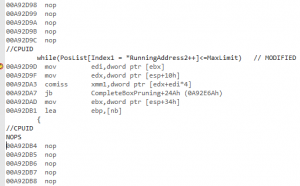
Now, as far as the disassembly is concerned, the changes are a bit hard to follow. The code got re-arranged (check out the position of “call operator delete” in versions 3 and 4 for example) and in its default form the disassembly is a bit obscure. Nonetheless, using the NOPS macro around the while instruction reveals that our change had the desired effect: one of the two comparisons clearly vanished.

More importantly, the benefits were not just theoretical. We also see the performance increase in practice:

Office PC:

Complete test (brute force): found 11811 intersections in 815456 K-cycles.
78703 K-cycles.
77667 K-cycles.
78142 K-cycles.
86118 K-cycles.
77456 K-cycles.
77916 K-cycles.
77156 K-cycles.
78100 K-cycles.
81364 K-cycles.
77259 K-cycles.
86848 K-cycles.
79394 K-cycles.
81877 K-cycles.
80809 K-cycles.
84473 K-cycles.
81347 K-cycles.
Complete test (box pruning): found 11811 intersections in 77156 K-cycles.

Home PC:

Complete test (brute force): found 11811 intersections in 781900 K-cycles.
82811 K-cycles.
81905 K-cycles.
82147 K-cycles.
81923 K-cycles.
82156 K-cycles.
81878 K-cycles.
82289 K-cycles.
82125 K-cycles.
82474 K-cycles.
82050 K-cycles.
81945 K-cycles.
82257 K-cycles.
81902 K-cycles.
81834 K-cycles.
82587 K-cycles.
82360 K-cycles.
Complete test (box pruning): found 11811 intersections in 81834 K-cycles.

The gains are summarized here:

Note that this optimization will only work if the input bounding boxes do not already contain our sentinel value - otherwise there would be no way to distinguish between the sentinel value and a regular value.

This is the first incidence of a rather common trend while optimizing code: the loss of genericity. Sometimes to make the code run faster, you need to accept some compromises or limitations compared to a fully “generic” implementation.

In this case, the limitation enforced by the optimization is that input bounding boxes cannot contain FLT_MAX. This is not a big problem in practice: usually only planes have infinite bounding boxes, and you can always make them use FLT_MAX/2 instead of FLT_MAX if needed. So this limitation is easy to accept. Sometimes they are a lot more debatable.

What we learnt:

Identify “useless” parts of the code that don’t contribute to the results, then eliminate them.

A less generic function can often run faster.

And that’s already it for this part, short and sweet.

GitHub code for part 4

Part 3: don’t trust the compiler

We now look at the “CompleteBoxPruning” function for the first time. This is my code but since I wrote it 15 years ago, it’s pretty much the same for me as it is for you: I am looking at some foreign code I do not recognize much.

I suppose the first thing to do is to analyze it and get a feeling for what takes time. There is an allocation:

Then a loop to fill that buffer:

Then we sort this array:

And then the rest of the code is the main pruning loop that scans the array and does overlap tests:

After that we just free the array we allocated, and return:

Ok, so, we can forget the allocation: allocations are bad and should be avoided if possible, but on PC, in single-threaded code like this, one allocation is unlikely to be an issue - unless not much else is happening. That leaves us with basically two parts: the sorting, and the pruning. I suppose this makes total sense for an algorithm usually called either “sweep-and-prune” or “sort-and-sweep” – the “box pruning” term being again just how I call this specific variation on the theme: single sorting axis, direct results, no persistent data.

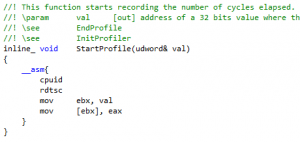
So first, let’s figure out how much time we spend in the sorting, and how much time in the pruning. We could use a profiler, or add extra rdtsc calls in there. Let’s try the rdtsc stuff. That would be an opportunity for me to tell you that the code in its current form will not compile for x64, because inline assembly is forbidden there. So the profiler functions for example do not compile:

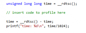
This is easy to fix though: these days there is a __rdtsc() intrinsic that you can use instead, after including <intrin.h>. Let’s try that here. You can include the header and write something like this around the code you want to measure:

If we apply this to the different sections of the code, we get the following results:

Allocation:
time: 3
time: 1
time: 1
time: 1
time: 1
time: 1
time: 1
time: 1
time: 1
time: 1
time: 1
time: 1
time: 1
time: 1
time: 1
time: 1

Remember that we looped several times over the “CompleteBoxPruning” function to get more stable results. Typically what happens then is that the first call is significantly more expensive than the other ones, because everything gets pulled in the cache (i.e. you get a lot more cache misses than usual). When optimizing a function, you need to decide if you want to optimize for the “best case”, the “average case”, or the “worst case”.

The best case is when everything is nicely in the cache, you don’t get much cache misses, and you can focus on things like decreasing the total number of instructions, using faster instructions, removing branches, using SIMD, etc.

The worst case is the first frame, when cache misses are unavoidable. To optimize this, you need to reduce the number of cache misses, i.e. decrease the size of your structures, use more cache-friendly access patterns, use prefetch calls judiciously, etc.

The average case is a fuzzy mix of both: in the real world you get a mixture of best & worst cases depending on what the app is doing, how often the function is called, etc, and at the end of the day, on average, everything matters. There is no right answer here, no hierarchy: although it is good practice to “optimize the worst case”, all of it can be equally important.

At this point the main thing is to be aware of these differences, and to know approximately if the optimization you’re working on will have an impact on the worst case or not. It is relatively common to work on a “best case” optimization that seems wonderful “in the lab”, in an isolated test app, and then realize that it doesn’t make any actual difference once put “in the field” (e.g. in a game), because the cost becomes dominated by cache misses there.

For now we are in the lab, so we will just be aware of these things, notice that the first frame is more expensive, and ignore it. If you think about it too much, you never even get started.

Sorting (static):
time: 686
time: 144
time: 139
time: 145
time: 138
time: 138
time: 138
time: 148
time: 139
time: 137
time: 138
time: 138
time: 137
time: 138
time: 146
time: 144

The sorting is at least 140 times more expensive than the allocation in our test. Thus, as expected, we’re just going to ignore the allocation for now. That was only a hunch before, but profiling confirms it was correct.

The first frame is almost 5 times more expensive than the subsequent frames, which seems a bit excessive. This comment explains why:

The code is using my old radix sort, which has a special trick to take advantage of temporal coherence. That is, if you keep sorting the same objects from one frame to the next, sometimes the resulting order will be the same. Think for example about particles being sorted along the view axis: their order is going to be roughly the same from one frame to the next, and that’s why e.g. a bubble-sort can work well in this case - it terminates early because there is not much work needed (or no work at all indeed) to get from the current ordering to the new ordering. The radix sort uses a similar idea: it starts sorting the input data using the sorted ranks from the previous call, then notices that the ranks are still valid (the order hasn’t changed), and immediately returns. So it actually skips all the radix passes. That’s why the first frame is so much more expensive: it’s the only frame actually doing the sorting!

To see the actual cost of sorting, we can remove the static keyword. That gives:

Sorting (non static):
time: 880
time: 467
time: 468
time: 471
time: 471
time: 470
time: 469
time: 469
time: 499
time: 471
time: 471
time: 490
time: 470
time: 471
time: 470
time: 469

That’s more like it. The first frame becomes more expensive for some reason (maybe because we now run the ctor/dtor inside that function, i.e. we allocate/deallocate memory), and then the subsequent frames reveal the real cost of radix-sorting the array. The first frame is now less than 2X slower, i.e. the cost of cache misses is not as high as we thought.

In any case, this is all irrelevant for now, because:

Pruning:
time: 93164
time: 94527
time: 95655
time: 93348
time: 94079
time: 93220
time: 93076
time: 94709
time: 93059
time: 92900
time: 93033
time: 94699
time: 94626
time: 94186
time: 92811
time: 95747

There it is. That’s what takes all the time. The noise (the variation) in the timings is already more expensive than the full non-static radix sorting. So we will just put back the static sorter and ignore it entirely for now. In this test, questions like “is radix sort the best choice here?” or “shouldn’t you use quick-sort instead?” are entirely irrelevant. At least for now, with that many boxes, and in this configuration (the conclusion might be different with less boxes, or with boxes that do not overlap each-other that much, etc), the sorting costs nothing compared to the pruning.

And then we can look at the last part:

Deallocation:
time: 4
time: 3
time: 3
time: 3
time: 6
time: 3
time: 3
time: 3
time: 3
time: 3
time: 3
time: 3
time: 3
time: 3
time: 3
time: 3

Nothing to see here, it is interesting to note that the deallocation is more expensive than the allocation, but this is virtually free anyway.

So, analysis is done: we need to attack the pruning loop, everything else can wait.

Let’s look at the loop again:

There isn’t much code but since we have a lot of objects (10000), any little gain from any tiny optimization will also be multiplied by 10000 - and become measurable, if not significant.

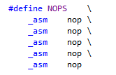
If you look at the C++ code and you have no idea, you can often switch to the disassembly in search of inspiration. To make it more readable, I often use a NOP macro like this one:

And then I wrap the code I want to inspect between nops, like this for example:

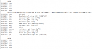
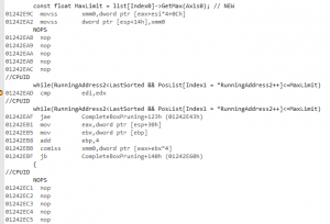
It allows me to isolate the code in the assembly, which makes it a lot easier to read:

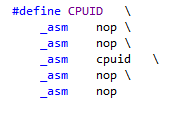
Note that the nops don’t prevent the compiler from reorganizing the instructions anyway, and sometimes an instruction you want to monitor can still move outside of the wrapped snippet. In this case you can use the alternative CPUID macro which puts a serializing cpuid instruction in the middle of the nops:

It puts more restrictions on generated code and makes it easier to analyze, but it also makes things very slow - in our case here it makes the optimized loop slower than the brute-force loop. It also sometimes changes the code too much compared to what it would be “for real”, so I usually just stick with nops, unless something looks a bit fishy and I want to double-check what is really happening.

Now, let’s look at the disassembly we got there.

While decorating the code with nops does not make everything magically obvious, there are still parts that are pretty clear right from the start: the cmp/jae is the first comparison (”while(RunningAddress2<LastSorted”) and the comiss/jb is the second one (”&& PosList[Index1 = *RunningAddress2++]<=list[Index0]->GetMax(Axis0))”).

Now the weird bit is that we first read something from memory and put it in xmm0 (”movss xmm0,dword ptr [eax+esi*4+0Ch]“), and then we compare this to some other value we read from memory (”comiss xmm0,dword ptr [eax+ebp*4]“). But in the C++ code, “list[Index0]->GetMax(Axis0)” is actually a constant for the whole loop. So why do we read it over and over from memory? It seems to me that the first movss is doing the “list[Index0]->GetMax(Axis0)”. It’s kind of obvious from the 0Ch offset in the indexing: we’re reading a “Max” value from the bounds, they start at offset 12 (since the mins are located first and they’re 4 bytes each), so that 0Ch must be related to it. And thus, it looks like the compiler decided to read that stuff from memory all the time instead of keeping it in a register.

Why? It might have something to do with aliasing. The pointers are not marked as restricted so maybe the compiler detected that there was a possibility for “list” to be modified within the loop, and thus for that limit value to change from one loop iteration to the next. Or maybe it is because “Index0″ and “Axis0″ are not const.

Or something else.

I briefly tried to use restricted pointers, to add const, to help the compiler see the light.

I failed.

At the end of the day, the same old advice remained: don’t trust the compiler. Never ever assume that it’s going to “see” the obvious. And even if yours does, there is no guarantee that another compiler on another platform will be as smart.

To be fair with compilers, they may actually be too smart. They might see something we don’t. They might see a perfectly valid (yet obscure and arcane) reason that prevents them from doing the optimization themselves.

In any case whatever the reason we reach the same conclusion: don’t rely on the compiler. Don’t assume the compiler will do it for you. Do it yourself. Write it this way:

And suddenly the disassembly makes sense:

The load with the +0Ch is now done before the loop, and the code between the nops became smaller. It is not perfect still: do you see the line that writes xmm0 to the stack ? (”movss dword ptr [esp+14h],xmm0″). You find it again a bit later like this:

So the compiler avoids the per-loop computation of MaxLimit (yay!) but instead of keeping it in one of the unused XMM registers (there are plenty: the code only uses one at this point), it writes it once to the stack and then reloads it from there, all the time (booh!).

Still, that’s enough for now. By moving the constant “MinLimit” and “MaxLimit” values out of the loops, in explicit const float local variables, we get the following timings:

Office PC:

Complete test (brute force): found 11811 intersections in 819967 K-cycles.
89037 K-cycles.
98463 K-cycles.
95177 K-cycles.
88952 K-cycles.
89091 K-cycles.
88540 K-cycles.
89151 K-cycles.
91734 K-cycles.
88352 K-cycles.
88395 K-cycles.
99091 K-cycles.
99361 K-cycles.
91971 K-cycles.
89706 K-cycles.
88949 K-cycles.
89276 K-cycles.
Complete test (box pruning): found 11811 intersections in 88352 K-cycles.

Home PC:

Complete test (brute force): found 11811 intersections in 781863 K-cycles.
96888 K-cycles.
93316 K-cycles.
93168 K-cycles.
93235 K-cycles.
93242 K-cycles.
93720 K-cycles.
93199 K-cycles.
93725 K-cycles.
93145 K-cycles.
93488 K-cycles.
93390 K-cycles.
93346 K-cycles.
93138 K-cycles.
93404 K-cycles.
93268 K-cycles.
93335 K-cycles.
Complete test (box pruning): found 11811 intersections in 93138 K-cycles.

The gains are summarized here:

“Delta” and “Speedup” are computed between current version and previous version. “Overall X factor” is computed between current version and the base version (version 2).

The base version is version2 to be fair, since version1 was the same code, just not using the proper compiler settings.

The code became faster. On the other hand the total number of instructions increased to 198. This is slightly irrelevant though: some dummy instructions are sometimes added just to align loops on 16-byte boundaries, reducing the number of instructions does not always make things faster, all instructions do not have the same cost (so multiple cheap instructions can be faster than one costly instruction), etc. It is however a good idea to keep an eye on the disassembly, and the number of instructions used in the inner loop still gives a hint about the current state of things, how much potential gains there are out there, whether an optimization had any effect on the generated code, and so on.

What we learnt:

Don’t trust the compiler.

Don’t assume it’s going to do it for you. Do it yourself if you can.

Always check the disassembly.

That’s enough for one post.

Next time we will stay focused on these ‘while’ lines and optimize them further.

GitHub code for part 3

Part 2 - compiler options

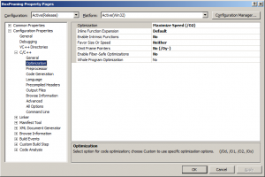
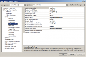
After converting the project, the default compiler options for the Release configuration are as follows (click to expand):

These are basically the only options affecting performance, if we ignore a few additional ones in the linker. After some years programming, you get a feeling for which ones of these options are important, and which ones are not.

So… what do you think, optimization experts?
Which one of these will make the most difference here?

For me, looking at that list, the suspicious ones that should be changed immediately are the following:

Inline Function Expansion: Default

Enable C++ Exceptions: Yes (/EHsc)

Enable Enhanced Instruction Set: Not Set

Floating Point Model: Precise (/fp:precise)

These guys are the usual suspects, as far as I’m concerned.

But let’s test this.

—

We first change the “Inline Function Expansion” option from “Default” to “Only __inline (/Ob1)”

Results:

Complete test (brute force): found 11811 intersections in 837222 K-cycles.

Complete test (box pruning): found 11811 intersections in 96230 K-cycles.

In general, inlining has a strong impact on performance, and there would be a need for an entirely separate blog post about the art of inlining. But in this specific case, it does not make any difference: the “Default” setting works well enough. The disassembly is the same 202 instructions as before so it did not change anything.

Note that it does not mean nothing gets inlined. “Default” does not mean “no inlining“. If you really disable inlining with the “Disabled /Ob0” option, you get the following results:

Complete test (brute force): found 11811 intersections in 1155114 K-cycles.

Complete test (box pruning): found 11811 intersections in 174538 K-cycles.

That is quite a difference. So clearly, inlining is one of the important things to get right, and in this specific case the default option is already right.

Good.

Now, we switch inlining back to “Default” and move on to the next option.

—–

This time we disable exceptions (“Enable C++ Exceptions: No”).

Results:

Complete test (brute force): found 11811 intersections in 817837 K-cycles.

Complete test (box pruning): found 11811 intersections in 95789 K-cycles.

It appears that disabling exceptions has a noticeable effect on the brute-force implementation, but no clear effect on the box-pruning function.

The disassembly shows the same 202 instructions as before, so the small performance gain is not actually here, it’s just noise in the results. It is important to check the disassembly to confirm that the “optimization” actually changed something. Otherwise you can often see what you want to see in the results…

Well, exceptions usually add a tiny overhead for each function, and it can accumulate and add up to “a lot” (relatively speaking). But we don’t have a lot of functions here, and as we just saw before with inlining, the few functions we have are properly inlined. So it makes sense that disabling exceptions in this case does not change much.

Worth checking though. Don’t assume. Check and check and check.

—–

Next, we turn exceptions back on (to measure the effect of each option individually) and then we move on to this:

Enable Enhanced Instruction Set: Not Set

This one is interesting. The default is “Not Set” but if you look at the disassembly so far, it is clearly using some SSE registers (for example xmm0). So it turns out that by default, the compiler uses SSE instructions these days. Which explains why switching to /arch:SSE2 gives these results:

Complete test (brute force): found 11811 intersections in 829134 K-cycles.

Complete test (box pruning): found 11811 intersections in 96448 K-cycles.

Again it appears that the option has a small effect on the brute-force code (if this isn’t just noise), and no effect on the box-pruning code. And indeed, the disassembly shows the same 202 instructions as before.

Now, as an experiment, we can switch back to regular x87 code with the /arch:IA32 compiler flag (”Enable Enhanced Instruction Set : No Enhanced Instructions”). This gives the following results:

Complete test (brute force): found 11811 intersections in 921893 K-cycles.

Complete test (box pruning): found 11811 intersections in 110605 K-cycles.

Ok, so that makes more sense: using SSE2 does in fact have a clear impact on performance, it’s just that the default “Not Set” option was actually already using it. That’s a bit confusing, but at least the results now make sense.

While we are looking at these results, please note how enabling the SSE2 compiler flag only provides modest gains, from ~110000 to ~97000: that’s about a 10% speedup only. This is again why we didn’t enable that compile flag back in PhysX 2.x. Contrary to what naive users claimed online, using the flag does not magically make your code 4X faster.

—–

Finally, we focus our attention on the Floating Point Model, and switch it to /fp:fast. You might guess the results by now:

Complete test (brute force): found 11811 intersections in 825688 K-cycles.

Complete test (box pruning): found 11811 intersections in 96115 K-cycles.

And yes, the disassembly is exactly the same as before. Frustrating.

—–

At that point I got tired of what looked like a pointless experiment. I just quickly setup the remaining options with my usual settings, compiled, and…

…the code got measurably faster:

Complete test (brute force): found 11811 intersections in 817855 K-cycles.

Complete test (box pruning): found 11811 intersections in 93208 K-cycles.

Like, a 100% reproducible good 3000 K-Cycles faster.

And the speedup was not imaginary, it was indeed reflected in the disassembly: 192 instructions.

What…

After a short investigation I discovered that the only compiler option that made any difference, the one responsible for the speedup was “Omit Frame Pointers“.

…the hell?

So, experts, did you predict that?

I did not.

This was doubly surprising to me.

The first surprise is that /O2 (which was enabled by default in Release, right from the start) is supposed to include /Oy, i.e. the “Omit Frame Pointers” optimization.

But this link explains the problem:

“The /Ox (Full Optimization) and /O1, /O2 (Minimize Size, Maximize Speed) options imply /Oy. Specifying /Oy– after the /Ox, /O1, or /O2 option disables /Oy, whether it is explicit or implied.”

So, the issue is that the combo box in the compiler options exposes “No (/Oy-)”, which is an explicit “disable” command rather than a “use whatever is the default”. So as the MSDN says, it overrides and undoes the /O2 directive. Oops.

The second surprise for me was that it had such a measurable impact on performance: about 5%. Not bad for something that wasn’t even on my radar. To be fair this issue doesn’t exist with 64-bit builds (as far as I know), so maybe that’s why I never saw that one before. According to the MSDN /Oy frees up one more register, EBP, for storing frequently used variables and sub-expressions. Somehow I didn’t realize that before, and it certainly explains why things get faster.

—–

Ok!

Compiler options: checked!

Other than that, I removed some obsolete files from the project, but made no code changes. This version is now going to be our base version against which the next optimizations will be measured.

For reference, this was my best run on the office PC:

Complete test (brute force): found 11811 intersections in 819814 K-cycles.
102256 K-cycles.
93092 K-cycles.
92885 K-cycles.
99537 K-cycles.
93146 K-cycles.
93325 K-cycles.
95795 K-cycles.
97573 K-cycles.
97606 K-cycles.
98829 K-cycles.
97040 K-cycles.
95197 K-cycles.
98149 K-cycles.
93226 K-cycles.
93008 K-cycles.
95254 K-cycles.
Complete test (box pruning): found 11811 intersections in 92885 K-cycles.

And on the home PC:

Complete test (brute force): found 11811 intersections in 781996 K-cycles.
102578 K-cycles.
98972 K-cycles.
98898 K-cycles.
99183 K-cycles.
98920 K-cycles.
98823 K-cycles.
98948 K-cycles.
99047 K-cycles.
99132 K-cycles.
98822 K-cycles.
98975 K-cycles.
100701 K-cycles.
98892 K-cycles.
99025 K-cycles.
99294 K-cycles.
98981 K-cycles.
Complete test (box pruning): found 11811 intersections in 98822 K-cycles.

The progress will be captured in this table:

What we learnt:

The default performance-related compiler options in Release mode are pretty good these days, but you can still do better if you go there and tweak them.

Next time, we will start looking at the code and investigate what we can modify. That is, we will start the proper optimizations.

GitHub code for part 2

Part 1 - The setup

Back in 2002 I released a small “box pruning” library on my website. Basically, this is a “broadphase” algorithm: given a set of input bounds (AABBs - for Axis Aligned Bounding Boxes), it finds the subset of overlapping bounds (reported as an array of overlapping pairs). There is also a “bipartite” version that finds overlapping boxes between two sets of input bounds. For more details about the basics of box pruning, please refer to this document.

Note that “box pruning” is not an official term. That’s just how I called it some 15 years ago.

Since then, the library has been used in a few projects, commercial or otherwise. It got benchmarked against alternative approaches: for example you could still find it back in Bullet 2.82’s “Extras\CDTestFramework” folder, tested against Bullet’s internal “dbVt” implementation. People asked questions. People sent suggestions. And up until recently, people sent me results showing how their own alternative broadphase implementation was faster than mine. The last time that happened, it was one of my coworkers, somebody sitting about a meter away from me in the office, who presented his hash-grid based broadphase which was “2 to 3 times faster” than my old box pruning code.

That’s when I knew I had to update this library. Because, of course, I’ve made that code quite a bit faster since then.

Even back in 2002, I didn’t praise that initial implementation for its performance. The comments in there mention the “sheer simplicity”, explicitly saying that it is “probably not faster” than the other competing algorithms from that time. This initial code was also not using optimizations that I wrote about later in the SAP document, e.g. the use of “sentinels” to simplify the inner loop. Thus, clearly, it was not optimal.

And then of course, again: it’s been 15 years. I learnt a few things since then. The code I write today is often significantly better and faster than the code I wrote 15 years ago. Even if my old self would have had a hard time accepting that.

So, I thought I could write a series of blog posts about how to optimize that old implementation from 2002, and make it a good deal faster. Like, I don’t know, let’s say an order of magnitude faster as a target.

Sounds good?

Ok, let’s start.

For this initial blog post I didn’t do any real changes, I am just setting up the project. The old version was compiled with VC6, which I unfortunately don’t have anymore. For this experiment I randomly picked VC11.

Here is a detailed list of what I did:

• Converted the project from Visual Studio 6 to Visual Studio 2012. I used the automatic conversion and didn’t tweak any project settings. I used whatever was enabled after the conversion. We will investigate the compiler options in the next post.
• Made it compile again. There were some missing loop indices in the radix code, because earlier versions of Visual Studio were notoriously not properly handling the scope in for loops (see /Zc::forScope). Other than that it compiled just fine.
• Moved the files that will not change in these experiments to a shared folder outside of the project. That way I can have multiple Visual Studio projects capturing various stages of the experiment without copying all these files in each of them.
• Added a new benchmark. In the old version there was a single test using the “CompleteBoxPruning” function, with a configuration that used 5000 boxes and returned 200 overlapping pairs. This is a bit too small to properly stress test the code, so I added a new test that uses 10000 boxes and returns 11811 intersections. That’s enough work to make our optimizations measurable. Otherwise they can be invisible and lost in the noise.
• In this new test (”RunPerformanceTest” function) I loop multiple times over the “BruteForceCompleteBoxTest” and “CompleteBoxPruning” tests to get more stable results (recording the ‘min’). Reported timing values are divided by 1024 to get results in “K-Cycles”.
• I also added a validity test (”RunValidityTest” function) to make sure that the two functions, brute-force and optimized, keep reporting the same pairs.

And that’s about it. There are no modifications to the code otherwise for now; it is the same code as in 2002.

The initial results are as follows, on my home PC and my office PC. The CPU-Z profiles for both machines are available here:

Home PC: pierre-pc

Office PC: pterdiman-dt

Note that they aren’t really “killer” machines. They are kind of old and not super fast. That’s by design. Optimizing things on the best & latest PC often hides issues that the rest of the world may suffer from. So you ship your code thinking it’s fast, and immediately get reports about performance problems from everybody. Not good. I do the opposite, and (try to) make the code run fast on old machines. That way there’s no bad surprises. For similar reasons I test the results on at least two machines, because sometimes one optimization only works on one, and not on the other. Ideally I could / should have used entirely different platforms here (maybe running the experiments on consoles), but I’m not sure how legal it is to publish benchmark results from a console, so, maybe next time.

Home PC:

Complete test (brute force): found 11811 intersections in 795407 K-cycles.
102583 K-cycles.
102048 K-cycles.
101721 K-cycles.
101906 K-cycles.
101881 K-cycles.
101662 K-cycles.
101768 K-cycles.
101693 K-cycles.
102094 K-cycles.
101924 K-cycles.
101696 K-cycles.
101964 K-cycles.
102000 K-cycles.
101789 K-cycles.
101982 K-cycles.
101917 K-cycles.
Complete test (box pruning): found 11811 intersections in 101662 K-cycles.

Office PC:

Complete test (brute force): found 11811 intersections in 814615 K-cycles.
106695 K-cycles.
96859 K-cycles.
97934 K-cycles.
99237 K-cycles.
97394 K-cycles.
97002 K-cycles.
96746 K-cycles.
96856 K-cycles.
98473 K-cycles.
97249 K-cycles.
96655 K-cycles.
102757 K-cycles.
96203 K-cycles.
96661 K-cycles.
107484 K-cycles.
104195 K-cycles.
Complete test (box pruning): found 11811 intersections in 96203 K-cycles.

The “brute force” version uses the unoptimized O(N^2) “BruteForceCompleteBoxTest” function, and it is mainly there to check the returned number of pairs is valid. I only report one performance number for this case - we don’t care about it.

The “box pruning” version uses the “CompleteBoxPruning” function, that we are going to optimize. As we can see here, this initial implementation offered quite decent speedups already - not bad for something that was about 50 lines of vanilla C++ code.

For the “complete box pruning case” I make the code run 16 times and record the minimum time. I am going to report the 16 numbers from the 16 runs though, to show how stable the machines are (i.e. do we get reproducible results or is it just random?), and to show the cost of the first run (which is usually more expensive than the subsequent runs, so it’s a worst-case figure).

These results are out-of-the-box after the automatic project conversion. Needless to say, this is compiled in Release mode.

If you want to replicate these numbers and get stable benchmark results from one run to the next, make sure your PC is properly setup for minimal interference. See for example the first paragraphs in this post .

For now I will only focus on the “CompleteBoxPruning” function, completely ignoring its “BipartiteBoxPruning” counterpart in my reports. All optimizations will be equally valid for the bipartite case, but there will be enough to say and report with just one function for now. The companion code might update and optimize the bipartite function along the way though - I’ll just not talk about it.

The initial disassembly for the function has 202 instructions. We are going to keep a close eye on the disassembly in this project.

That’s it for now.

Next time, we will play with the compiler options and see what kind of speedup we can get “for free”.

GitHub code for part 1