Coder Corner

Part 17 – PhysX lessons

In this series, we have been looking at fairly low-level optimizations so far. For example reducing the number of instructions, reducing the amount of cache-misses, aligning the data, switching to SIMD, etc. Grosso modo, we have improved the implementation of an algorithm.

But that was only the first part. In this post we start investigating the other side of the story: high-level optimizations, i.e. improvements to the algorithm itself.

Multi Box Pruning

In part 1, I briefly explained where “box-pruning” came from. The details are available in the sweep-and-prune (SAP) document that I wrote a decade ago now. That paper also explains the issues with the traditional SAP algorithm, and introduces the “multi-SAP” idea to address them.

The box-pruning algorithm we have been optimizing so far is also a SAP variant, and as such it suffers from similar issues. For example box pruning also suffers from “useless interactions with far away objects”, as described in page 17 of the SAP document. This is easy to see: imagine a vertical stack of equally-sized boxes, with either Y or Z as the up/vertical axis. Our code projects the boxes on the X axis. So all “projected” values end up equal (all min values are the same, all max values are the same). The “pruning power” of the first loop drops to zero. The second loop basically degenerates to our brute-force version. This is of course an extreme example that would not happen exactly as-is in practice, but the important point is that mini-versions of that example do happen all over the place in regular cases, making the broadphase less efficient than it could be.

The “multi-SAP” solution used a grid over the 3D world. Objects were assigned to grid cells, and a regular SAP was used in each cell. By design faraway objects then ended up in faraway cells, reducing the amount of aforementioned useless interactions.

We added something similar to multi-SAP in PhysX starting from version 3.3. It was called “MBP”, for Multi Box Pruning. As the name suggests, it was basically the multi-SAP idea applied to a box-pruning algorithm rather than applied to a regular incremental sweep-and-prune. It turns out that algorithmic improvements to SAP also work for box-pruning.

The PhysX implementation differs from the Multi-SAP implementation detailed in the SAP document. For example it does not use a grid of non-overlapping cells. Instead, it needs user-provided broadphase regions, which can overlap each other. And each object can belong to an arbitrary number of cells. But other than these implementation details, the basics are the same as what I described ten years ago: the overlaps are found separately for each region, they are added to a shared pair manager structure, and some extra management code is needed to deal with objects crossing regions.

In our box pruning project here, we do not have any API for updating or removing objects from the structures: we effectively do the PhysX “add object” operations each time. This has pros and cons.

The bad thing about this is that it is not optimal in terms of performance. In all our timings and tests so far, we have always been recomputing the exact same set of overlaps each time – each “frame” if you want. A good broadphase would take advantage of this, notice that objects have not changed from one call to the next, and only the first call would actually compute the overlaps. Subsequent calls would be either free (as for the incremental SAP in PhysX) or at least significantly cheaper (as for MBP in PhysX).

On the other hand, the good thing about this is that we do not need the previously mentioned “extra management code” from MBP in our little project here. To replicate the “add object” codepath from MBP, all we would need is some grid cells and a pair manager, i.e. for example a hash-map. Recall that so far we added overlapping pairs to a simple dynamic array (like an std::vector<Pair>). In MBP, an object touching two separate grid cells is added to both cells. So when computing the overlaps in each cell individually, it is possible to find the same overlapping pair multiple times. Some mechanism is needed to filter out duplicates, and in PhysX we do this by adding pairs to a shared hash-map / hash-set.

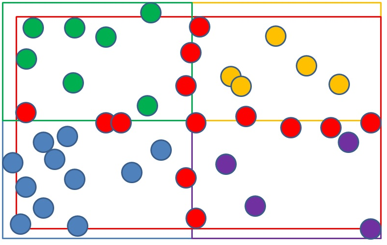
We do not have user-defined broadphase regions in this project, but we could try to compute some of them automatically. Here is how it would work in 2D:

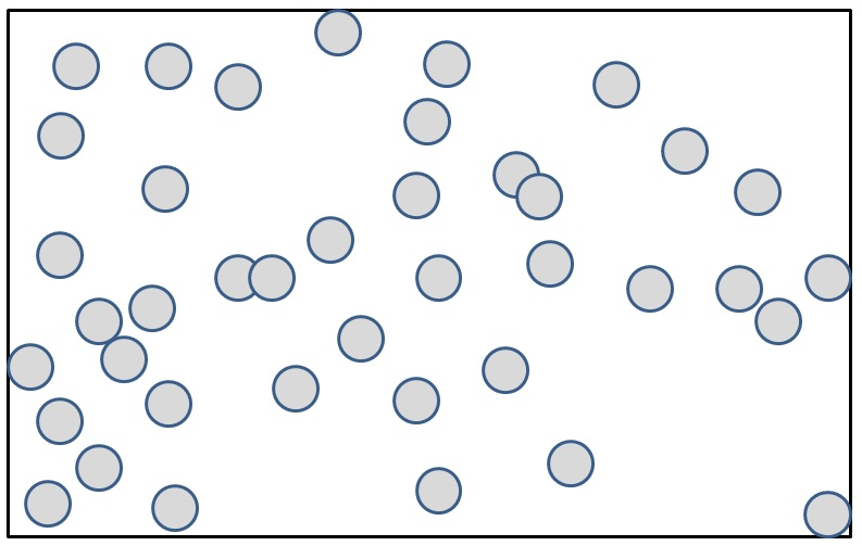
a) Start with a bunch of objects (the blue spheres). Compute the black bounding box around them.

Picture 1: compute the AABB around all objects

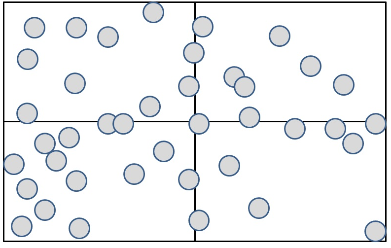
b) Subdivide the bounding box computed in the first step. This gives 4 broadphase regions.

Picture 2: subdivide the AABB into 4 regions

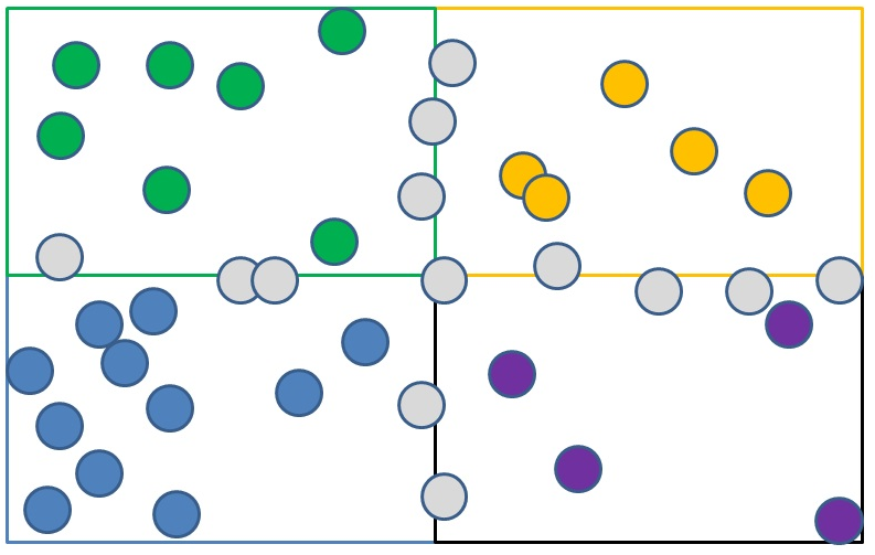
c) Classify objects depending on which region they fall in. Green objects go into the 1st region, yellow objects into the 2nd region, blue objects into the 3rd region, magenta objects into the 4th region.

Picture 3: assign objects to regions

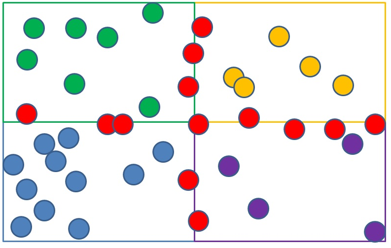
d) The remaining red objects touch multiple regions. In PhysX using MBP, each red object is duplicated in the system, added to each region it touches.

Picture 4: objects touching multiple regions are duplicated

To find the overlaps, we then perform 4 “completeBoxPruning” calls (one for each region). Colliding pairs are added to a shared hash-map, which by nature filters out duplicates. So for example a pair of touching red objects, like the one overlapping the green and blue regions in the picture, will be reported twice by both the green and blue broadphase regions. But since we add the pair to a shared (unique) hash-map, the second addition has no effect.

So we could replicate this in our box-pruning project. We could implement a hash-map (or reuse one that I released on my website years ago) and give this a try. But adding the same objects to different regions also leads to increased memory usage. And the resulting code quickly becomes unpleasant.

So instead, in this project we’re going to try something different.

Bucket pruner

There is another interesting data structure in PhysX called a “bucket pruner”. This is used in the context of scene queries rather than broadphase (i.e. raycasts, overlap tests, etc). Long story short, we needed something that was faster to build than a regular AABB tree, while providing some speedup compared to testing each objects individually.

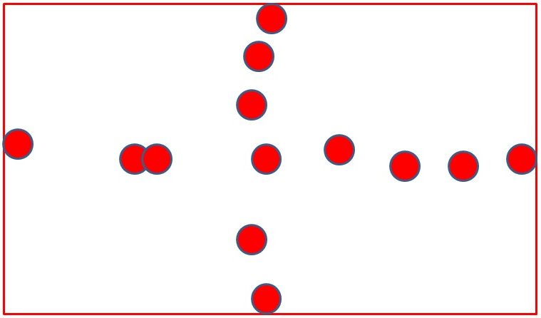
Roughly speaking, it is built exactly like what we just described before. The 4 previously defined broadphase regions are what we call the “natural buckets”. But the structure handles the red objects in a different way: they are not duplicated and added to existing regions; instead they go to a special 5th bucket named “cross bucket”.

Picture 5: put duplicated objects in their own region

It is called “cross bucket” (or boundary bucket) because objects inside it often form a cross-like shape. It also contains objects that cross a boundary, so the name has a double meaning.

Picture 6: the cross bucket

In PhysX the classification process is then repeated again for each bucket (with special subdivision rules for the cross-bucket). This is done recursively a fixed number of times. At the end of the day the bucket pruner is a mix between a BVH and a spatial-partitioning structure: we compute bounds around objects as in a BVH, but we divide the resulting space in equally-sized parts as in a spatial partitioning structure (e.g. a quadtree). Since we do not do any clever analysis to find the best splitting points, and because we only recurse a small fixed amount of times, the whole thing is quick to build – much quicker than a regular AABB tree for example.

Now, how does that help us for box-pruning?

This is where all the pieces of the puzzle come together, and my cunning plan is revealed.

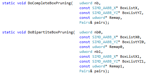
Do you remember part 1, where I mentioned the BipartiteBoxPruning function? This is the companion to the CompleteBoxPruning function we have been optimizing so far. CompleteBoxPruning finds overlaps within a set of objects. BipartiteBoxPruning finds overlap between two separate sets of objects. As we mentioned in part 1, all the optimizations we have been doing up to this point are equally valid for the bipartite case. And while I did not put any emphasis on it, I kept updating the bipartite case as well along the way.

That was by design. I knew I was going to need it eventually.

It turns out that we can take advantage of the bipartite case now, to optimize the complete case. The trick is simply to run 4 CompleteBoxPruning calls for the 4 natural buckets (as in MBP), and then run 5 additional calls:

• 1 CompleteBoxPruning call to find overlaps within the 5th bucket
• 4 BipartiteBoxPruning calls to find overlaps between the 5th bucket and buckets 1 to 4

Because of the extra calls it might be less efficient than the MBP approach overall (I did not actually try both here), but this new alternative implementation has two advantages over MBP:

• There is no need to duplicate the objects. We can simply reshuffle the same input arrays into 5 sections, without the need to allocate more memory.
• There is no need for a hash-map. This approach does not generate duplicate pairs so we can keep adding our colliding pairs to our simple dynamic array like before.

Overall this approach is much simpler to test in the context of our box-pruning project, so that is why I selected it.

Implementation in our project

First, we allocate a little bit more space than before for our split boxes. Recall that in version 16 we did something like this:

The +1 in the BoxListX allocation was initially added in version 4, to make space for a sentinel value. The extra +5 was added later when we unrolled the loops that many times. And then the +1 in BoxListYZ is actually unnecessary: it appeared when we split the boxes in version 9c (we allocated the same amount of “X” and “YZ” parts), but we only need sentinels in the X buffer so we could allocate one less element in the YZ buffer.

Now, for version 17 we are going to create 5 distinct sections within these buffers (one for each bucket). Each bucket will be processed like our arrays from version 16, i.e. each of them needs to have sentinel values. Thus for 5 buckets we need to allocate 5 times more sentinels than before, i.e. a total of 30 extra entries in the X buffer. The YZ buffer does not need extra space however, thanks to our previous observation that allocating one extra entry there was in fact not needed. The resulting code looks like this:

—

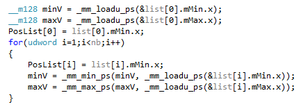
Next, we compute the initial bounding box (AABB) around the objects. This is the black bounding box in picture 1). We already had a loop over the source data to compute “PosList” in version 16, so computing an extra bounding box at the same time is cheap (it does not introduce new cache misses or new branches):

The only subtle issue here is that the last SIMD load on the last box reads 4 bytes past the end of the source array. This can crash if the last allocated entry was exactly at the end of a memory page. The simplest way to address this is to allocate one more dummy box in the source array.

—

Once the AABB is computed, we can subdivide it as shown in picture 2). We are not doing any clever analysis to find the split points: we just take the middle of the box along Y and Z. The main box-pruning code projects the boxes on the X axis already (hardcoded in Part 5), so we ignore the X axis for our broadphase regions, and we split along the two other axes:

—

These two limit values and the initial bounding box implicitly define the 4 bounding boxes around the natural buckets. With this knowledge we can then classify boxes, and assign each of them to a bucket. Because we ignore the X axis, we effectively deal with 2D boxes here. A box fully contained within one of the 4 natural buckets is given an ID between 0 and 3. A box crossing a bucket’s boundary ends up in the cross bucket, with ID 4.

The classification is a fairly straightforward matter:

Each box is tested against the previously computed limits. In sake of completeness, let’s reverse-engineer the code. Let’s call B the main black box from Picture 1).

We see from the way it is computed that limitY is B’s center value on axis Y. We then compare it to the incoming box’s min and max Y values. We compare Y values together, that is consistent and good. If leftPart is true, it means the incoming box is fully on the left side of the split, i.e. the box does not cross the Y boundary. But if rightPart is true, the box is fully on the right side of the split. It should not be possible for leftPart and rightPart to be both true at the same time.

Similarly, limitZ is B’s center value on axis Z. We compare it to the incoming box’s min and max Z values, which is also consistent and correct. If lowerPart is true, it means the incoming box is fully on the lower side of the split, i.e. the box does not cross the Z boundary. But if upperPart is true, the box is fully on the upper side of the split. It should not be possible for lowerPart and upperPart to be both true at the same time.

The classification is then:

• leftPart && lowerPart => the box is fully in region A
• leftPart && upperPart => the box is fully in region B
• rightPart && lowerPart => the box is fully in region C
• rightPart && upperPart => the box is fully in region D

In any other case, the box is crossing at least one boundary, and thus ends up in region E – the cross bucket. Doing these comparisons is a bit costly so instead we compute a 4-bit mask from the test results and use it as an index into a small look-up table. The disassembly shows that using a table avoids branches (this is similar to what we covered in version 8):

00AE3B90 movss xmm0,dword ptr [edx]
00AE3B94 xor ecx,ecx
00AE3B96 comiss xmm2,dword ptr [edx+0Ch]
00AE3B9A lea edx,[edx+18h]
00AE3B9D seta cl
00AE3BA0 xor eax,eax
00AE3BA2 lea esi,[esi+4]
00AE3BA5 add ecx,ecx
00AE3BA7 comiss xmm0,xmm2
00AE3BAA movss xmm0,dword ptr [edx-1Ch]
00AE3BAF seta al
00AE3BB2 or ecx,eax
00AE3BB4 xor eax,eax
00AE3BB6 add ecx,ecx
00AE3BB8 comiss xmm1,dword ptr [edx-10h]
00AE3BBC seta al
00AE3BBF or ecx,eax
00AE3BC1 xor eax,eax
00AE3BC3 add ecx,ecx
00AE3BC5 comiss xmm0,xmm1
00AE3BC8 seta al
00AE3BCB or ecx,eax
00AE3BCD movzx eax,byte ptr [ecx+0B04250h]
00AE3BD4 mov dword ptr [esi-4],eax
00AE3BD7 inc dword ptr [esp+eax*4+0A0h]
00AE3BDE dec edi
00AE3BDF jne CompleteBoxPruning+1B0h (0AE3B90h)

It may not be optimal but it is good enough for now. The table is simple enough to derive. We organize the mask like this:

lowerPart | upperPart | leftPart | rightPart

Thus we get:

• 0000 - region E
• 0001 - region E
• 0010 - region E
• 0011 - leftPart/rightPart both set, not possible
• 0100 - region E
• 0101 - upperPart && rightPart => region D
• 0110 - upperPart && leftPart => region B
• 0111 - leftPart/rightPart both set, not possible
• 1000 - region E
• 1001 - lowerPart && rightPart => region C
• 1010 - lowerPart && leftPart => region A
• 1011 - leftPart/rightPart both set, not possible
• 1100 - lowerPart/upperPart both set, not possible
• 1101 - lowerPart/upperPart both set, not possible
• 1110 - lowerPart/upperPart both set, not possible
• 1111 - leftPart/rightPart both set, not possible

—

Once the bucket indices are available for all boxes, BoxXListBuffer and BoxListYZBuffer are filled with sorted boxes, like we did in version 16. The only difference is that boxes are stored per bucket there: all boxes of bucket 0 (sorted along X), then all boxes of bucket 1 (sorted along X), and so on. This part is just simple pointer and counter book-keeping, no major issue. Just remember to write all the necessary sentinels at the end of each section within the array.

—

At this point the data is ready and we can do the actual pruning. In version 16, we only had one “complete box pruning” function running there. In version 17 we will need to run multiple “complete box pruning” calls on 5 distinct parts of the arrays, and additional “bipartite box pruning” calls. Thus we first copy the corresponding code into separate functions:

This is the same code otherwise as in version 16; we just move it to separate functions.

—

Finally, we do the sequence of complete and bipartite pruning calls that we mentioned in a previous paragraph:

In these two for loops, i is the bucket index. We first find overlaps within each of the 5 buckets (the first for loop), then we find overlaps between bucket 4 (the cross bucket) and the 4 first natural buckets.

That’s it.

As promised, the modifications we made to try this new approach are somewhat minimal. There is no need to introduce a hash-map or more complicated memory management, it’s all rather simple.

Admittedly, the approach does not guarantee performance gains compared to version 16. We could very well find degenerate cases where all objects end up in the same bucket. But even in these bad cases we would effectively end up with the same as version 16, with a modest overhead introduced by the bounding box computation and box classification. Not the end of the world. Most of the time objects are distributed fairly homogeneously and the approach gives clear performance gains.

It certainly does in our test project, in any case:

What do we get?

We see clear gains compared to our previous version 16 on all machines. This is the only “apples-to-apples” comparison we have here, since the pruning code is effectively the same in both versions. So we only measure the effect of our high-level optimization here, and we can conclude that it does work.

Perhaps more interestingly, version 17 is also faster than version 15b on all tested machines. That is, our C++ SSE2 version is now faster than our best assembly SSE2 version. This is pretty good because it was the opposite before: version 15b was faster than version 16 on all machines. Of course the comparison is a bit unfair here, and we could port the high-level optimization to version 15b to get some gains there as well. However we would need to write the whole bipartite function in assembly, so that is a lot more work than what we did for the C++ version. Exercise left to the readers and all that (or to cough Fabian cough :)).

Finally, on machines that support it, the AVX version remains the fastest. Or so it seems.

The trap of the unique benchmark

In this series we have consistently made one cardinal mistake. Something that experienced programmers know is a very bad idea. We ignored the first rule of optimization 101:

Use more than one benchmark.

You need to start somewhere of course, and we’ve gone a long way with our unique test scenario in this project – so a single benchmark does provide value, and it is certainly better than no benchmark at all.

However, using a single benchmark has its perils. By nature it tends to test a single codepath, a single configuration, a single way to navigate through your code. And of course, there is absolutely no guarantee that a different scenario produces the same performance profile. There is no guarantee that a specific optimization helps in all cases. Change the input data, and maybe you reach a different conclusion. Maybe your algorithm does not scale. Maybe something helps for a large number of objects, but hurts for a small number of them. Maybe one optimization helps when a lot of boxes do overlap, but hurts when the same boxes are disjoint. And so on. There is a huge amount of combinations, codepaths, configurations, which are as many traps one can fall into.

And thus, at some point one must start using more than one benchmark. In PhysX for example, I remember creating 4 or 5 different benchmarks just to test a single box-vs-triangle overlap function (similar to my blog post here). The function had multiple codepaths, some with early exits, and I created a separate benchmark for each of them. This is impossible to do for a full physics engine, but that is the spirit.

Now this is a toy project here so I will not go crazy with the number of scenarios we support: I will just add one more, to prove a point.

Go back to the main source file where we define the test. Find this line:

const udword NbBoxes = 10000;

Then just add a zero:

const udword NbBoxes = 100000;

What happens when we test ten times more boxes?

Well the first thing one notices is that our initial versions become insufferably slow. The code now finds and reports 1144045 pairs and it brings our first versions to their knees. It is so bad that our profiling function cannot even measure the time properly: our naïve version only returned the lower 32bit part of the TSC counter (which is a 64bit value), and the initial code is so slow that we wrap around, producing meaningless timings.

So I will just ignore the first versions and show the results for latest ones. This is now for 100000 boxes:

While the timings generally follow the same pattern as in our previous test with less boxes, we clearly see that version 17 is now the fastest on all tested machines. The high-level optimization was more effective for a large number of boxes than it was for a “small” number of them.

I did not do a thorough analysis to explain why but generally speaking it is true that simple brute-force versions can be faster than smarter versions when you only have a small amount of items to process. In our case we added some overhead to compute the initial bounding box and classify boxes into buckets, which is an O(n) part, while the following pruning loops are not O(n) (as you can see with the timings: we multiplied the amount of boxes by 10 but the time it takes to process them grew by more than 10). The relative cost of the “preparation” part compared to the “pruning” part has an impact on which version is eventually the fastest.

And then again, there are different codepaths within the pruning part itself (how many overlap tests do we end up with? How many of them report a hit?) and increasing the amount of boxes might add some pressure on a codepath that was previously less traveled.

In short: one benchmark is not enough.

The bipartite case

We mentioned that until now, all our improvements to the complete case were equally valid for the bipartite case. But the optimizations for the bipartite case will be slightly different in this version, since we cannot exactly replicate there what we did for the complete case.

What we can do is the following:

• Compute buckets for both incoming sets of objects A and B (similar to what we did before)
• Compute buckets’ bounds (this is new, we did not need them in the complete case)
• Do a bipartite box pruning call between each bucket of A and each bucket of B, if their respective bounds overlap.

And with this, we can wrap this part up.

What we learnt:

Low-level optimizations are important but not the only thing to care about. High-level algorithmic optimizations are equally important.

One benchmark is not enough. Some optimizations might work in some scenarios, while being detrimental in others. Use multiple benchmarks with various workloads and various configurations, to stress multiple codepaths.

We can make the complete-box-pruning codepath faster using the bipartite-box-pruning codepath. But we cannot make the bipartite case faster using the complete case. For the first time the bipartite case needed specific changes.

We reached our goal of being faster than the AVX version, at least in some scenarios.

So… are we finally done?

Ah.

Not really.

We just opened the door to high-level optimizations, so we still have a long way to go.

GitHub code for version 17 is here.